Fun With Random Numbers: Random Projection

The Fantastic Claim

Let’s say you have a set of 1000 points in a 10,000 dimensional space. These points could be the brightness of pixels from 100x100 grayscale images. Or maybe they’re the term counts of the 10,000 most frequent terms in a document from a corpus of documents. Whatever they are, each point has 10,000 dimensions.

10,000 dimensions is hard to work with, so you’re interested in reducing the dimensionality of your data. The goal of such a reduction would be to make the points easier to work with (have fewer than 10,000 dimensions), but preserve the relevant structure so you can treat the reduced dimensional data as if it were the high dimensional data (analyze it, machine learn it, whatever).

One piece of the structure you might be interested in preserving is the distance between the points. What does it mean to preserve distance? Let’s pick a percentage called ε and say that we want all distances between points calculated in the low dimensional space to be no more than ε% different from the distance between the same points calculated in the original high dimensional space. In pseudo math you might say that good dimensionality reductions lead to distances that obey D_LowDimension= D_{High Dimension} ± ε% for all points.

So now we can get to the JL lemma’s fantastic claim.

The JL lemma says that the number of dimensions you need in your lower dimensional space is completely independent of the number of dimensions in the original space. Your original data could be 10,000-dimensional or 10,000,000,000-dimensional, and the number of dimensions you need in the lower dimensional space in order to preserve distance depends only on the number of points and our boundary ε. The formula for the number of dimensions you need is:

OK, let’s stop and take a breath. This result is absolutely-positively-100%-certified-grade-A-what-the-hell-is-up-with-the-universe to me. It’s beautiful and it makes my brain hurt. When I first thought about it I couldn’t do anything but stand up and pace around for a while. Take a minute or two to do the same.

The Fantastic Method

Welcome back.

Brace yourself. Even more fantastic than the claim that such dimensionality reductions exist and that they don’t depend on the dimensionality of the original space, is the method of doing such a reduction. Here’s the code…

N = 10000 #The Number of dimensions in the original space
n = 1000  #The number of dimensions in the low dimensional space

random_matrix = matrix(rnorm(N * n), 0, 1), N, n)) / sqrt(m) #The magical random matrix.
X = GetData() #returns a nPoints x N matrix of your data points

X_projected = X %*% random_matrix

It’s…just random numbers. To do one of these good dimensionality reductions, you just sample an N × n matrix from the standard normal distribution and multiply. IT’S JUST RANDOM NUMBERS. Probably time for another walk and think.

SRSLY?

Welcome back, again. At this point I was at a total loss. We only need ln(NumberOfPoints) dimensions to have a good projection, and doing the projection is just sampling a random matrix and a matrix-multiply? Like, for real? This is a true fact? I tried to understand the proofs here but they’re a tad inscrutable (and not just to me). It happens. I’m an engineer with some math background, not a mathematician. The next best thing is to just try it, right? The claim is so simple to test, and the method so simple to implement, that if I just run the code enough times I can quiet down my brain’s utter disbelief and maybe this can become a tool in my toolbox.

OK, let’s do it.

library(tidyverse)
N = 10000 #The Number of dimensions in the original space
m = 1000  #The number of points in the dataset
epsilon = .1

X = matrix(rnorm(m * N, 100, 10), m, N) #Let's just pick some normal random data.
distX = dist(X) %>% as.matrix() #This is the distance matrix in the original space.

n = as.integer(ceiling(log(m) / epsilon ^ 2)) + 1 #The number of dimensions in the projected space.

random_matrix = matrix(rnorm(N * n, 0, 1), N, n) / sqrt(n) #The magical random matrix
random_matrix = matrix(rnorm(N * n, 0, 1), N, n) / sqrt(n) #See it's totally random, really there's nothing special about it.
random_matrix = matrix(rnorm(N * n, 0, 1), N, n) / sqrt(n) #Look, the deck is really shuffled. Completely random. No tricks.

X_projected = X %*% random_matrix #Project the points into the lower dimension.
distX_projected = dist(X_projected) %>% as.matrix() #The distance matrix in the projected space.

distances = data.frame(Distance = as.numeric(distX),
                       ProjectedDistance=as.numeric(distX_projected))

We’ve projected the original 10,000 dimensions down to 692 dimensions. We expect that all the distances are distorted by less than 10%. Let’s look at a histogram of the distortion of the distances…

distances %>%
  filter(Distance > 0.0) %>% #Ignore the distance from a point to itself.
  mutate(Distortion = (ProjectedDistance - Distance) / Distance) %>% 
  sample_frac(.1) %>%
  ggplot(aes(Distortion)) +
  geom_histogram(bins=40) + 
  geom_vline(xintercept = epsilon, color = "red", lty = 2) +
  geom_vline(xintercept = -epsilon, color = "red", lty = 2) + 
  labs(title = "Distribution of Distortion") + 
  theme(plot.title=element_text(size=22),
        axis.text.x=element_text(size=14),
        axis.text.y=element_text(size=14))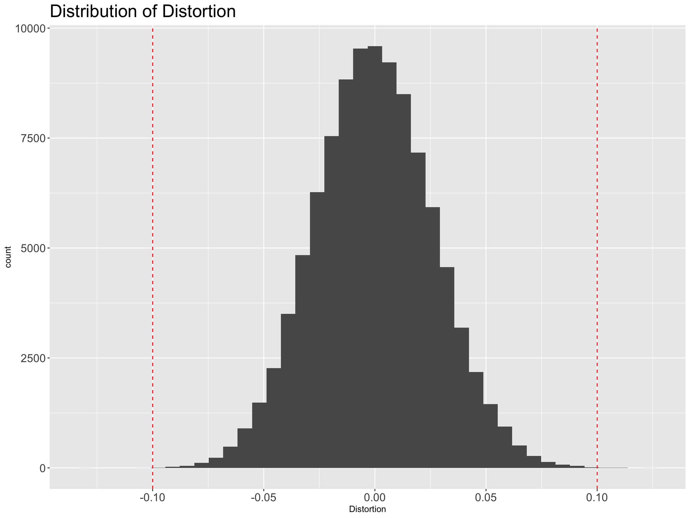 

And we see that they’re basically all in range. Fantastic.